I recently had to estimate the range of a species for different time periods from data that were aggregated to the township level. The area of these townships can vary by hundreds to thousands of square kilometers. I decided to somehow find the 95% minimum convex polygon for each period. I was not contempt on using the centroid distance, because of the widely varying sizes of the polygons. However, the advantage of using the centroid is the short length of time it takes to calculate the pairwise distance between points compared to calculating the pairwise distance between polygon edges. For example, if I generate 1000 polygons and calculate the pairwise edge distance between them it takes 6 seconds, but only 0.3 seconds using the centroids. For 10,000 polygons it takes 681 and 3 seconds. This increase in processing time might not seem like much time, but I used 1000 polygons as an easy example. As you increase the number of polygons the computation time exponentially increases. In addition the memory usage also increase exponentially. When I compute the polygon edge distance for 1000 polygons the result only uses 4 mb, but for 10,000 polygons the result uses 381 mb of my virtual memory. There are many ways around these computation limits, but this is not the point of this entry. Keep in mind that these polygons are simple circles and are not complex in anyway, this means computations is fairly quick compared to more complex polygons.
Since I wanted to build my 95% mcp using the polygon edge distances I had to write my own R function. In my circumstance, I had to compute the pairwise distance of over 4000 complex polygons. I wrote a function that uses parallel computation and threading. In the following example, I did not write the code for parallel processing, I might make an entry on this topic later on in the year. In general, the script calculates the 95% minimum convex polygon using polygon edge distance. The R code is found below.
Since I wanted to build my 95% mcp using the polygon edge distances I had to write my own R function. In my circumstance, I had to compute the pairwise distance of over 4000 complex polygons. I wrote a function that uses parallel computation and threading. In the following example, I did not write the code for parallel processing, I might make an entry on this topic later on in the year. In general, the script calculates the 95% minimum convex polygon using polygon edge distance. The R code is found below.
|
First I created my fake data (Fig 1). There are 100 different spatial units with varying sizes. The coordinate were pulled from a uniform distribution, but the size were generated from a normal distribution with a large standard deviation.
Next I calculate the edge distance between each polygon and calculate the sum of the pairwise distance of each polygon. I then calculated the 95% probability cutoff using quantiles and identified polygons that had a sum distance smaller than this cutoff. These polygons are within the mcp. Fig 2 illustrates which polygons were within the 95% cutoff (green) and the ones that were not (red). I generated 100 random polygons and 5 were rejected from the mcp. Most of these are found at the boundary of the map near the right side. A small polygon is found on the lower left side, but you cannot see it because the mcp line overlaps it. It makes more sense when you look at the last figure.
I wanted to compare this 95% mcp generated from polygons to one generate from the centroids from these same polygons. I repeated the above, but this time I used the centroid distance. As expected, not all the same points were selected (Fig 3).
Finally, Fig 4 compares both methods. The blue line is the 95% mcp generated from polygons and the green line is generated from the centroids of these polygons. Both methods differ by 2 polygons, but agree on 3 polygons that shouldn't be included in the 95% mcp.
|
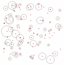
Fig 1
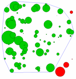
Fig 2
|
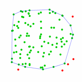
Fig 3
|
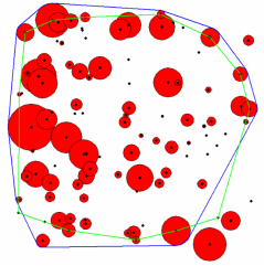
Fig 4
|
 RSS Feed
