Earlier I showed how to use Circuitscape in R. The only complications were to create your own CS .ini file and find the path to your CS .exe file. I wrote up a small script that compares Circuitscape's resistance distance to the random walk distance from the commuteDistance R 'gdistance' package. I also compare these two to the costDistance least-cost distance function from gdistance and the straight euclidean distance.
Essentially, the script simulates a landscape by generating spatially correlated random fields or in more fancy terms performing a unconditional Gaussian simulation. I adapted the code written by Santiago Beguería on his website. Check out his website If you want a nice tutorial on how to simulated spatially correlated data. After the landscape is simulated, a pair of random points is generated and all 4 algorithms calculate their distances between these points. These steps are repeated n times by switching the input to the lapply function at the end of the script. Right now it generates 1000 simulations. To plot the results I first standardized the data using the scale function.
Results Part 1
After simulating 1 landscape and 30 sites, all 4 methods performed 435 paired observation (n(n-1)/2). Resistance and commute distance had nearly a 1:1 linear relationship. Euclidean and least-cost distance also had a linear relationship. There is a exponential relationship between Euclidean distance and both resistance distance methods (resistance and commute distance). The samething is true for least-cost distance and both resistance distance methods.

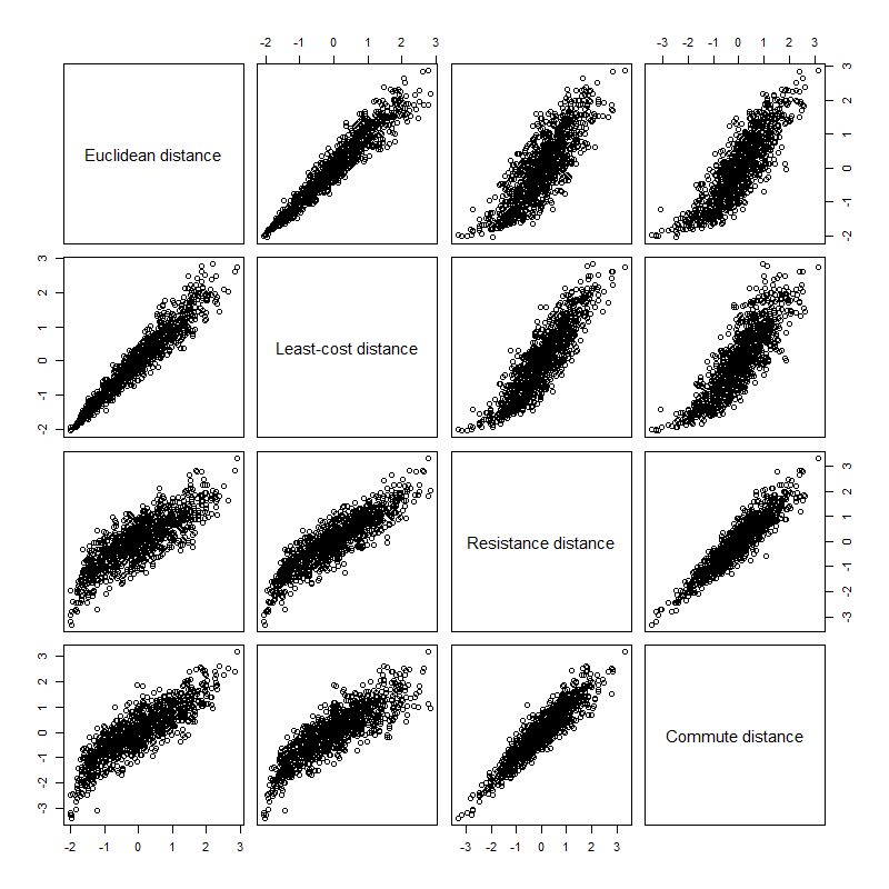
Results Part 2
After simulating 1000 different landscape and pairs of points the relationship between Euclidean/cost distance and Resistance/Commute distance becomes less clear. However, there is still a a linear trend between euclidean distance and Least-cost distance. Commute distance and resistance distance also still have a linear relationship. Euclidean distance still has a exponential relationship when we compare it to resistance and commute distance. Finally, least-cost distance still has a exponential relationship when we compare to resistance and commute distance.
After simulating 1000 different landscape and pairs of points the relationship between Euclidean/cost distance and Resistance/Commute distance becomes less clear. However, there is still a a linear trend between euclidean distance and Least-cost distance. Commute distance and resistance distance also still have a linear relationship. Euclidean distance still has a exponential relationship when we compare it to resistance and commute distance. Finally, least-cost distance still has a exponential relationship when we compare to resistance and commute distance.
 RSS Feed
